Customer Analytics
House price regression: what an R² of 0.77 really tells you
A linear regression built with discipline: log transformation, multicollinearity removed via VIF, significance pruning, four assumption checks and 10-fold cross-validation. The model explains around 77% of the variance - and reading the remaining metrics honestly matters more than the number itself.
Regression is considered the boring craft of data analysis - which is exactly why it is so good at showing where models fail in practice. Not at the algorithm, but at what happens before and after it: skewed target variables, features that measure the same thing, and metrics that sound better than they are. This project builds a classic OLS model on housing data and takes each of those points seriously.
The dataset
The basis is the well-known Boston housing dataset, a public educational dataset used in the MIT program: neighbourhood attributes such as crime rate (CRIM), nitric oxide levels (NOX), average number of rooms (RM), pupil-teacher ratio (PTRATIO) and the share of lower-status households (LSTAT), plus the median house price (MEDV) as the target.
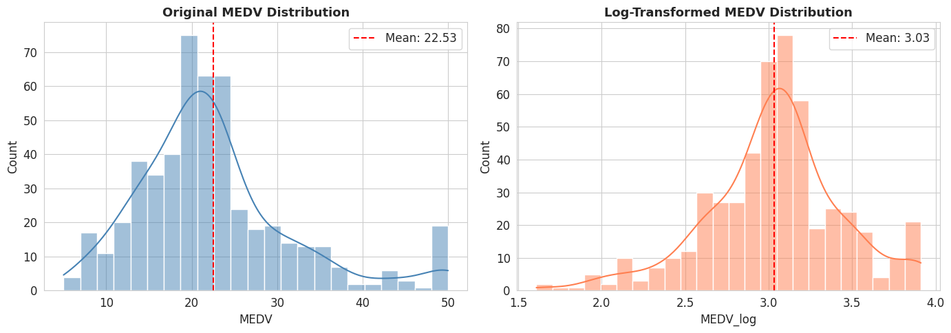
Two notes belong here, not at the end. First, this dataset is historically contested - the original version contains a race-related attribute, which is why it was removed from scikit-learn. The version used here does not contain that attribute; the work uses only the structural and environmental features listed above. The dataset serves as a methodological vehicle, not as a statement about housing markets. Second, the target variable is capped at 50 ($k) - every more expensive property is set to the same value. You can see it in the distribution, and it limits what the model can learn at the top end.
Preparation: straightening the target
The price distribution is clearly right-skewed. So the model targets not MEDV but log(MEDV) - a standard transformation that makes the distribution more symmetric and the assumptions of linear regression plausible in the first place.
Multicollinearity: which features tell the same story
Before modelling comes the question of whether features duplicate each other. The correlation matrix shows it clearly: RAD and TAX correlate at 0.91 - effectively the same information. NOX, INDUS and AGE are closely linked as well.
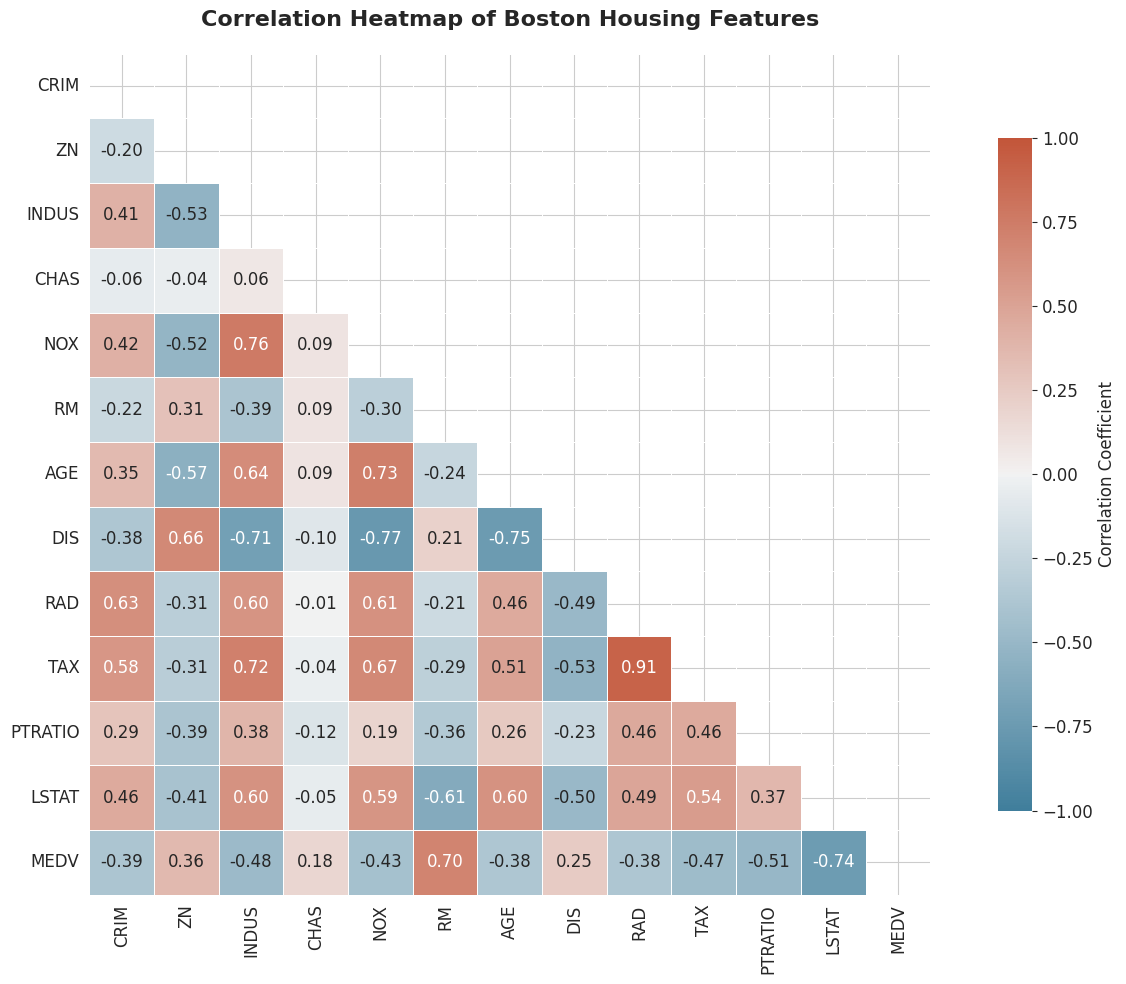
Confirmed by the Variance Inflation Factor (VIF), TAX was removed. In a second step ZN, AGE and INDUS dropped out because they were not significant in the model. The final model works with eight features: CRIM, CHAS, NOX, RM, DIS, RAD, PTRATIO, LSTAT.
Results
| Dataset | R² | Adj. R² | RMSE | MAE | MAPE |
|---|---|---|---|---|---|
| Training | 0.7672 | 0.7618 | 0.1955 | 0.1437 | 4.98% |
| Test | 0.7725 | 0.7581 | 0.1980 | 0.1513 | 5.26% |
RMSE, MAE and MAPE refer to the log-transformed target, not to dollar amounts.
What the analysis actually shows
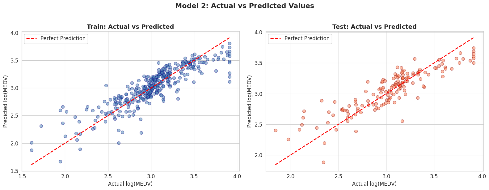
- No overfitting. Test R² (0.7725) is even marginally above the training value - the eight features generalise.
- The 5% MAPE is not a 5% price error. It is computed on the log scale. Turning it into "the model is 5% off on house prices" transfers a metric into a unit it was never measured in. The defensible statement remains: around 77% of the variance explained.
- Cross-validation is less calm than it looks. Across 10 folds the mean R² is 0.7291 with a spread of ±0.2322. The mean confirms the model; the spread says that individual splits run markedly worse - with 506 observations that is expected, and it is part of the result.
- The drivers are plausible, not causal. More rooms (RM) go with higher prices, a higher LSTAT share with lower ones. These are associations in 1970s neighbourhood data - not proof of effect, and certainly not a recommendation to act on.
The assumptions were checked, not assumed
A linear regression is only worth as much as its assumptions. All four were checked: the mean of the residuals (practically zero), homoscedasticity (constant error spread), the linearity of relationships via residuals against fitted values, and the normality of the error terms. Only then is interpreting the model permissible - in practice this is the step most often skipped.
Reproducibility & verification
The full code (EDA, preparation, VIF, both models, assumption checks, cross-validation) is in the companion repository: github.com/myBytesResearch/boston-house-price-prediction. The project was completed as coursework in the MIT Professional Education Applied AI and Data Science Program (verifiable certificate).