Research methodology
The second layer: what a regime model really delivers in lead time
We had announced that we would document the second model layer openly. Here it is: a hidden Markov model on the same four soft commodities, at the identical, pre-registered measurement endpoint as the GARCH baseline. The lead-time column looks spectacular. The real subject of this article is the question of which of these values you may trust, and why.
In the baseline article we showed that a classical GJR-GARCH-t passes the VaR discipline on ICE Cocoa, Coffee, Sugar and Cotton but delivers no early warning: the conditional volatility follows the move, it does not run ahead of it. The open question was whether a regime layer changes that.
The answer is a yes with an important caveat. Yes, the regime model fires ahead of all four examined episode onsets, at a controlled alarm rate, and for cocoa it marks a real market event three and a half months before the episode onset. But: the lead-time metric itself is more fragile than the numbers suggest, and part of what looks like confirmation is mechanics. We show openly what is which.
1 · The model and the protocol
The second layer is deliberately classical: a Gaussian hidden Markov model with three regimes (calm, elevated, stress) on the daily log returns, that is, the classical HMM formulation of the Baum-Rabiner line (Rabiner 1989), in which the returns are independently normally distributed given the state. For distinction: the regime switching established in econometrics after Hamilton 1989 is an HMM with an autoregressive emission structure; our variant is the simpler, more robust i.i.d. emission form. Markov-switching GARCH, in which the GARCH parameters themselves are state-dependent, is yet a third class and the next registered candidate (§5). The stress regime is defined as the state with the largest fitted variance. The signal is the strictly causal, filtered probability of the stress regime: on each day, only information up to that day enters, with no smoothing over the future.
The protocol is identical to the baseline, so that the comparison holds:
- same data snapshot, same four ICE continuous futures
- walk-forward with an expanding window, re-estimation every 21 trading days (about 179 re-estimations per commodity), fixed seed
- identical, pre-registered measurement endpoint for detection: EMA reference (lambda 0.94), sensitive operating point with a 10 % tolerated false-alarm rate, calibrated jointly across all four markets on the years 2019-2020, lead window 180 days
- no specification search per market: one specification, four commodities
The implementation, the configuration and the complete result files are in the companion repository
soft-commodities-forecast-benchmark
(src/benchmark/hmm_regime.py, src/benchmark/hmm_evaluate.py,
results/hmm_detection_evaluation.json).
2 · The result at the pre-registered endpoint
| Commodity | Episode | GARCH (layer 1) | HMM (layer 2) | HMM detection day |
|---|---|---|---|---|
| Cocoa | 2023/24 supply shock | no detection | 171 days | 2023-03-13 |
| Coffee | 2024 Brazil drought | 135 days | 169 days | 2024-03-15 |
| Sugar | 2023 India export curb | 178 days | 142 days | 2023-04-11 |
| Cotton | 2022 supply shock | 50 days | 179 days | 2021-11-02 |
Three reading aids for this table, before anyone copies it into a sales deck:
First: the alarm rate is controlled. Over the test years 2021-2024 the share of alarm days lies between 9.6 % and 13.1 %, consistent with the calibrated 10 % operating point. So the model does not shout constantly; when it fires, it is rare enough to mean something operationally.
Second: values near 180 days deserve mistrust. The lead window is 180 days long. A lead time of 179 days (cotton) means the alarm was already standing on the first day of the window, and that is not an early warning ahead of this event but the after-effect of the 2021 cotton rally with the Ukraine shock in its back. We therefore report this value as a window-edge finding, not as a detection. The same mistrust applies, in weaker form, to cocoa (171) and coffee (169) at the ratio endpoint; the harder test follows in the next section.
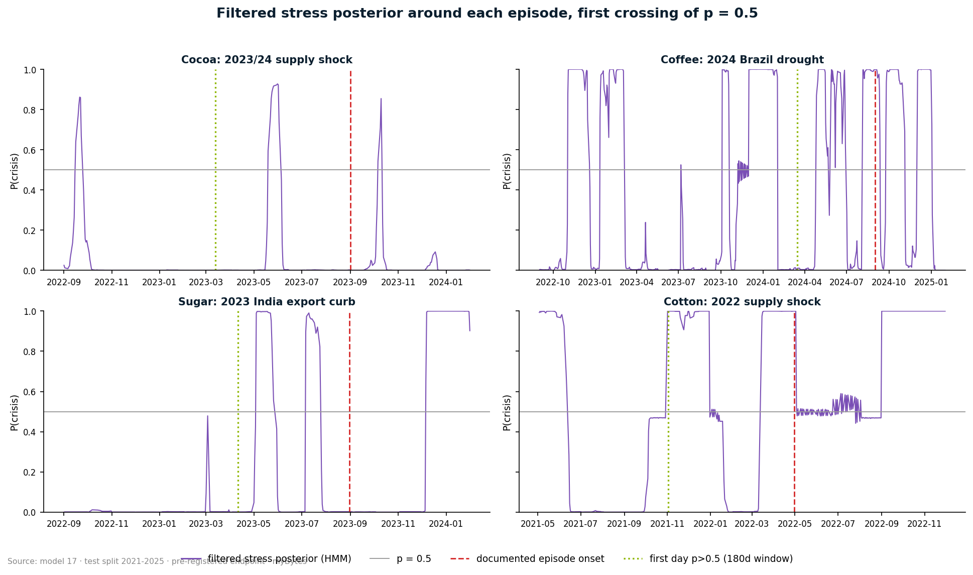
Third: the layer-1 column measures the evaluation mechanics, not GARCH as an early warner. The documented baseline statement is: the conditional volatility does not rise at the episode onsets, it follows the move. That the lead-time column nevertheless reports three of four detections for the same model is due to the first-crossing mechanics over long windows, with the same window-edge caveats as in layer 2. This is exactly why the full lead-time discussion belongs in this article and not in the baseline article: it is a property of the measurement procedure that can only be shown cleanly in the two-layer comparison.
3 · The most interesting single finding, honestly placed
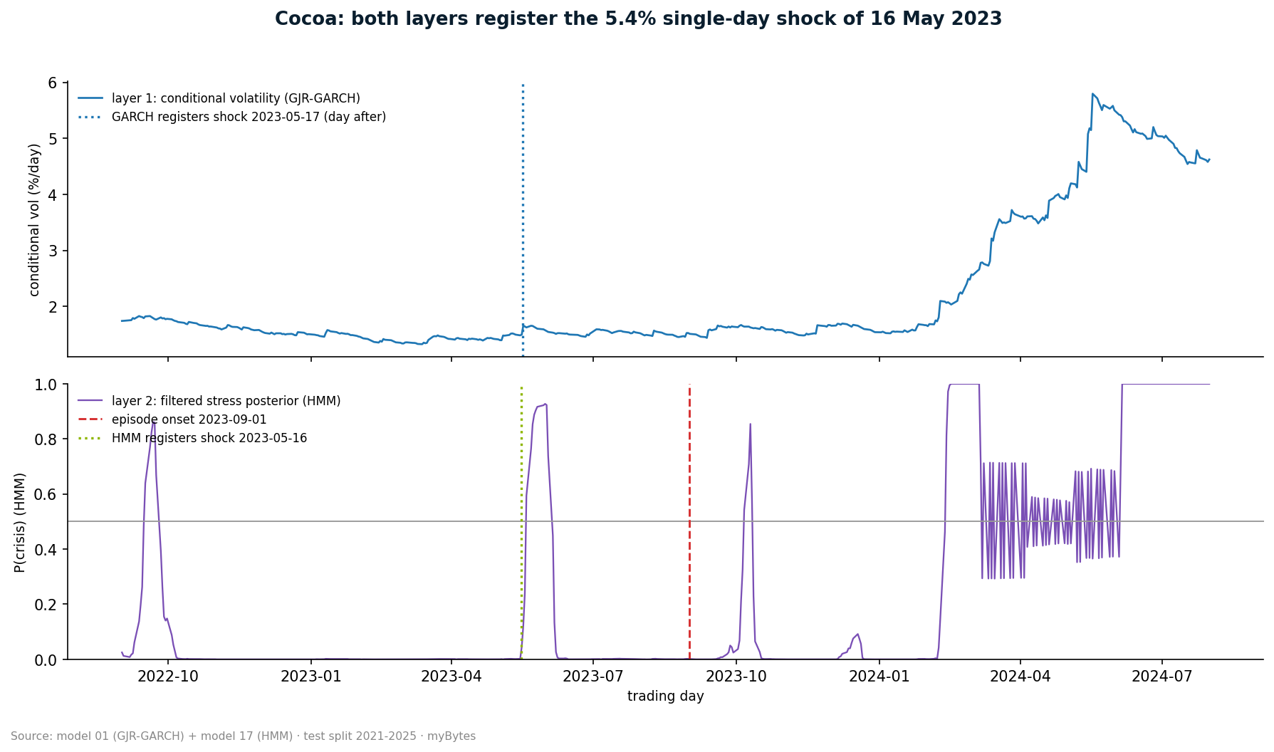
With a fixed probability threshold of 0.5 (pre-registered as a sensitivity evaluation), the regime model fires for cocoa on 16 May 2023: the filtered stress probability jumps from 0.10 to 0.84. The GARCH layer, in its single-market calibration, fires on 17 May 2023, one trading day later.
Before this becomes a legend, the honest mechanics: on 16 May 2023 the cocoa future fell 5.4 % in a single day. Both layers work on the same returns, and both react to large daily moves, the HMM on the day itself (the filter sees the spike immediately), the GARCH one day later (the conditional variance picks up after the shock). That both mark almost the same day is therefore not an independent cross-confirmation of two methods; it is the consistent registration of the same shock by two differently sluggish measurement instruments.
What the finding is actually worth: three and a half months before the documented episode onset, and eleven months before the all-time high, there was a real, sharp market event in cocoa, in the window in which the season's first deficit reports were circulating. Both layers make this event visible and datable. Whether it was causally the start of the episode or an isolated shock can only be answered by the fundamental layer (§6).
make reproduce and
python -m benchmark.hmm_evaluate.
Two further caveats belong here. The May signal is a short, sharp flare-up of one trading week; afterwards the model returns to the calm state until the episode onset; between detection and episode onset the stress probability is above 0.5 on only 5 % of days. Anyone who had traded on this signal in May 2023 would have needed patience. And: at the stricter threshold of 0.9, none of the four detections survives except the cotton window-edge finding. The event is real, but as a signal it is a whisper, not an alarm.
4 · When lead-time numbers deceive
This section is the reason the lead-time discussion deserves its own article. Three mechanisms can produce lead time without a model foreseeing anything:
- Window-edge hits. If the alarm is already standing on the first day of the lead window, the number does not measure the distance between signal and event but the window length. Recognizable by the lead time lying close to the maximum (cotton: 179 of 180).
- Predecessor events. In the commodity years 2022-2024 the episodes lay close together: Ukraine shock, sugar rally, cocoa deficit. An alarm in the lead window of event B can be the after-effect of event A. The detection on 11 March 2022 ahead of the cotton collapse in May is, with high probability, the Ukraine shock, not cotton.
- Calibration on non-calm reference years. Our thresholds are calibrated on 2019-2020, and the COVID spring of 2020 lies in that period. The thresholds are therefore conservative; the reported lead times are more likely under- than overstated. The effect thus biases against us, not for us, and remains documentation-worthy nonetheless.
The operational consequence: a single lead-time number is no proof of early-warning capability. A signal becomes dependable only through the combination of a controlled alarm rate, confirmation by a genuinely independent method (a different data source, not just a different model class) and an explanation of what the signal saw in substance. For cocoa May 2023 the alarm rate is controlled and the event is real and datable; the independent confirmation and the substantive explanation are outstanding and are the task of the fundamental layer. For cotton, none of the criteria is met.
5 · Steel-man: “three regimes are arbitrary, and HMMs are old”
The strongest counter-position: the number of regimes is a free choice, Markov-switching GARCH would be more elegant, and modern approaches (neural state-space models, foundation models) would beat both.
Three answers:
- The three-regime choice was fixed before the first run and was not adjusted based on results. That it is not optimized is not a flaw but the condition under which the results mean something. A sensitivity check over the number of regimes is marked as exploratory follow-up work.
- Old is an advantage here. Hamilton 1989 is forty years of method history with known weaknesses, and precisely for that reason we know where to look (label identification, EM convergence, both checked in the audit). A method whose breaking points are documented is worth more for a risk layer than a method whose breaking points nobody knows yet.
- The bar for any more complex candidate is now fixed: identical endpoint, identical protocol, and it must deliver the cocoa May signal without blowing up the alarm rate. Markov-switching GARCH is the next registered candidate.
6 · What this article does not do
- No new science. Methodologically there is nothing new here: the reactivity of GARCH is textbook knowledge, regime detection via HMM is Hamilton 1989, and the fragility of first-crossing lead times is known to the changepoint literature. The contribution of this work is the openly reproducible, pre-registered comparison setup across four markets with an identical endpoint, including the findings that speak against us. Anyone expecting a research breakthrough is in the wrong place; anyone who wants to see how to make early-detection claims audit-proof is in the right one.
- One stress episode per commodity. Four episodes across four markets are four data points. Every statement here is a statement about these four cases, not about soft-commodity crises in general.
- The episode definitions are retrospective. We know today which episodes were stress. A real-time system would not have had the episode list. The external anchors (ICCO deficit reports, India's export restrictions, the Brazil drought) are documented but do not replace prospective validation.
- No trading system. Neither the detections nor the lead times are buy, sell or hedging signals. The stack is a research test bench for the question of which signal layers hold under which conditions.
- COVID in the calibration window (see §4): conservative bias, documented, to be checked in follow-up work via an alternative reference window.
- The May signal is not explained, only observed. Whether the models in May 2023 saw the first deficit reports, positioning shifts or simply a lead move in prices is answered only by the fundamental layer (weather, export and inventory data), which is the next stage of the programme.
7 · Reading list
- Rabiner 1989, A Tutorial on Hidden Markov Models, the HMM foundation of the Baum-Rabiner line our specification follows.
- Hamilton 1989, A New Approach to the Economic Analysis of Nonstationary Time Series and the Business Cycle, regime switching in econometrics (HMM with an autoregressive emission structure).
- Hamilton/Susmel 1994, Autoregressive conditional heteroskedasticity and changes in regime, Markov-switching ARCH, the next registered candidate.
- Glosten/Jagannathan/Runkle 1993, the layer-1 baseline.
- Kupiec 1995 and Christoffersen 1998, the VaR discipline against which layer 1 was measured.
Related articles
- The Single-GARCH Limit on Soft Commodities, the layer-1 baseline whose announcement this article redeems.
- A Truth-Check Protocol for AI Research Output, the review procedure both articles passed through, including the audit that triggered the layer-1 correction.
Companion repository
myBytesResearch/soft-commodities-forecast-benchmark,
both layers in one repository: GJR-GARCH baseline and HMM regime module, identical walk-forward protocol,
pre-registered endpoint in configs/global.yaml, complete result files, make reproduce.
Private at publication time; the visibility flip to public is a separate, deliberate step.
Disclaimer
This article describes a model comparison from our own research practice on publicly available market data. It is neither investment nor hedging advice. The detection and lead-time values cited refer to a specific, pre-registered evaluation configuration and four historical episodes; they are not readily transferable to other markets, periods or configurations.